


A Beginner-Friendly Introduction To Improving Model Performance
Written by: Emmanuel Amoaku
In the realm of machine learning, building effective and accurate models is a constant pursuit. However, achieving optimal performance often requires fine-tuning various hyperparameters that govern the behaviour of the model. This process can be time-consuming and challenging, especially when dealing with complex datasets and models. Two powerful techniques that can aid in this venture are cross-validation and grid search. In this article, we’ll dive into these methods, exploring their theoretical foundations and practical applications, accompanied by code examples.
Cross-Validation: Assessing Model Performance Reliably
Cross-validation is a resampling technique used to evaluate the performance of a machine learning model on unseen data. It helps to estimate how well the model will generalize to new, previously unseen data, and ultimately aids in selecting the best model or hyperparameter configuration.
In traditional model evaluation, the dataset is typically split into a training set and a test set.
The model is trained on the training set and evaluated on the test set. However, this approach can lead to overfitting or underfitting if the test set is not representative of the underlying data distribution.
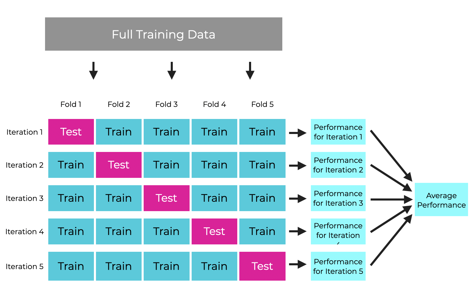
Cross-validation addresses this issue by repeatedly partitioning the dataset into different subsets for training and validation. The most common approach is k-fold cross-validation, where the dataset is divided into k equal-sized folds or subsets.
The model is then trained k times, each time using a different fold as the validation set and the remaining k-1 folds as the training set. The performance metrics (e.g., accuracy, F1-score, mean squared error) are computed for each fold, and the final performance estimate is calculated as the average of the k individual performance metrics.
In this example, we use scikit-learn’s cross_val_score function to perform 5-fold cross-validation on the iris dataset using a simple logistic regression model. Let’s start out by importing the necessary libraries:
from sklearn.model_selection import cross_val_score
from sklearn.linear_model import LogisticRegression
from sklearn.datasets import load_iris
from sklearn.metrics import accuracy_score
We then load the iris dataset using the load_iris() function from scikit-learn. The dataset is split into features (X) and target labels (y). The iris.data contains the feature values, and iris.target contains the corresponding class labels.
Load the iris dataset

iris = load_iris()

X, y = iris.data, iris.target
We create an instance of the LogisticRegression model from scikit-learn. This is the machine learning model we’ll be using for classification on the iris dataset.
Create a logistic regression instance
model = LogisticRegression()
We then perform 5-fold cross-validation using the cross_val_score function from scikit-learn. The function takes the following arguments:
⦁ model: The machine learning model to be evaluated (in this case, the LogisticRegression instance).
⦁ X: The feature data (iris.data).
⦁ y: The target labels (iris.target).
⦁ cv=5: This specifies that we want to perform 5-fold cross-validation.
⦁ scoring=’accuracy’: This indicates that we want to evaluate the model’s performance using the accuracy metric.
Perform 5-fold cross-validation

scores = cross_val_score(model, X, y, cv=5, scoring='accuracy')
The cross_val_score function splits the dataset into 5 folds, trains the model on 4 folds (80% of the data), and evaluates it on the remaining fold (20% of the data). This process is repeated 5 times, each time using a different fold as the test set. The function returns an array of scores, one for each fold.
Finally, we print the average cross-validation accuracy score by taking the mean of the scores array obtained from cross_val_score. The :.2f formats the output to display two decimal places.
Print the average cross-validation score

print(f"Average cross-validation accuracy: {scores.mean():.2f}")
Output
[]:
Average cross-validation accuracy: 0.97Grid Search: Automating Hyperparameter Tuning
While cross-validation helps evaluate model performance, grid search is a technique used to systematically search for the optimal combination of hyperparameters that maximize a model’s performance.
In machine learning models, hyperparameters are configuration settings that are not learned from the data during training but are set beforehand. Examples include the regularization strength (C) in logistic regression, the number of trees in a random forest, or the learning rate in a neural network.
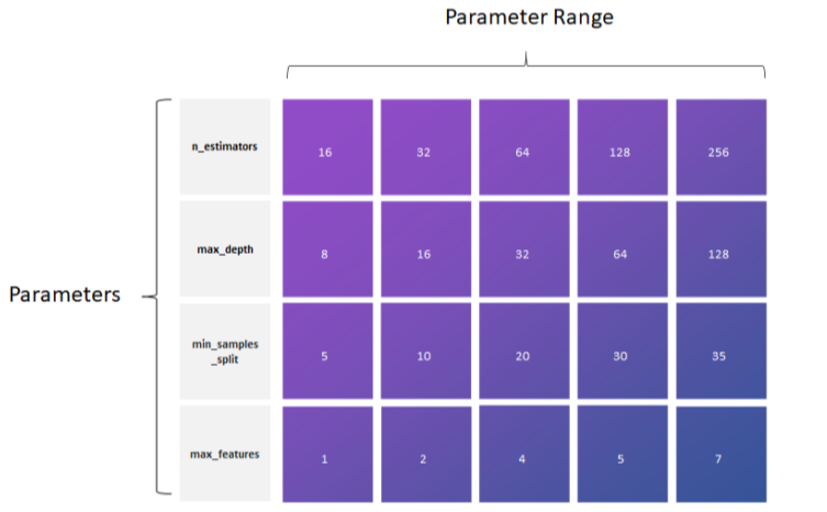
Grid search involves specifying a range of values for each hyperparameter of interest and evaluating the model’s performance for every possible combination of these values. This exhaustive search is typically performed using cross-validation to obtain a reliable estimate of the model’s performance for each hyperparameter combination.
For this example, GridSearchCV is used for performing grid search, SVC is the Support Vector Classifier model we’ll be using, load_digits is a function to load the digits dataset (a commonly used dataset for classification tasks), and accuracy_score is a metric for evaluating the model’s performance. We’ll start off by importing the necessary modules and functions from scikit-learn:
from sklearn.model_selection import GridSearchCV
from sklearn.svm import SVC
from sklearn.datasets import load_digits
from sklearn.metrics import accuracy_score
We then load the iris dataset using the load_digits() function from scikit-learn. The dataset is split into features (X) and target labels (y). The digits.data contains the feature values, and digits.target contains the corresponding class labels.
Load the digits dataset

digits = load_digits()

X, y = digits.data, digits.target
In the following section, we define the parameter grid for the grid search using a Python dictionary. The param_grid specifies the hyperparameters we want to tune and the values we want to explore for each hyperparameter. In this case, we’re tuning the kernel type (‘rbf’ or ‘poly’), the regularization parameter C (0.1, 1, or 10), and the kernel coefficient gamma (‘scale’ or ‘auto’).
Define the parameter grid for grid search
param_grid = {
'kernel': ['rbf', 'poly'],
'C': [0.1, 1, 10],
'gamma': ['scale', 'auto']
}
We create an instance of the SVC (Support Vector Classifier) model from scikit-learn. This is what we’ll be using for classification on the digits dataset.
Create a support vector machine instance

model = SVC()
We then create an instance of GridSearchCV with the following arguments:
⦁ model: The machine learning model to be optimized (in this case, the SVC instance).
⦁ param_grid: The parameter grid we defined earlier, specifying the hyperparameters and their values to explore.
⦁ cv=5: This specifies that we want to perform 5-fold cross-validation during the grid search process.
⦁ scoring=’accuracy’: This indicates that we want to evaluate the model’s performance using the accuracy metric.
Perform grid search
grid_search = GridSearchCV(model, param_grid, scoring='accuracy')

grid_search.fit(X, y)
The grid_search.fit(X, y) method performs the grid search on the entire dataset (X and y). It trains and evaluates the model with all possible combinations of hyperparameters and selects the best hyperparameter combination based on the specified scoring metric (accuracy in this case). Finally, we print the best hyperparameters found by the grid search (grid_search.best_params_).
Print the best hyperparameters and score

print(f"Best parameters: {grid_search.best_params_}")
Output []:
Best parameters: {'C': 10, 'gamma': 'scale', 'kernel': 'rbf'}Combining Cross-Validation and Grid Search for Optimal Model Performance
Cross-validation and grid search are often used in tandem to achieve the best possible model performance. The typical workflow involves:
⦁ Define the model and the hyperparameters to tune.
⦁ Specify the range of values for each hyperparameter (the grid).
⦁ Perform nested cross-validation:
⦁ Outer loop: Split the data into k folds for cross-validation.
⦁ Inner loop: For each fold in the outer loop:
⦁ Split the training data (k-1 folds) into a new training and validation set.
⦁ Perform grid search on the inner training set, evaluating each hyperparameter combination using the inner validation set.
⦁ Select the best hyperparameter combination based on the inner validation performance.
⦁ Train the model with the best hyperparameters on the entire training data (k-1 folds).
⦁ Evaluate the model on the outer loop’s test fold (the held-out fold).
⦁ Compute the overall performance metric by averaging the scores from all outer loop folds.
We start off by importing the necessary modules and functions from scikit-learn, including GridSearchCV for grid search, cross_val_score for cross-validation, SVC for the Support Vector Classifier model, load_digits to load the digits dataset, accuracy_score for evaluating the model’s accuracy, and StratifiedKFold for stratified cross-validation. We also import numpy for numerical operations.
from sklearn.model_selection import GridSearchCV, cross_val_score
from sklearn.svm import SVC
from sklearn.datasets import load_digits
from sklearn.metrics import accuracy_score
from sklearn.model_selection import StratifiedKFold
import numpy as np
We then load the iris dataset using the load_digits() function from scikit-learn. The dataset is split into features (X) and target labels (y).
Load the digits dataset

digits = load_digits()

X, y = digits.data, digits.target
We define the parameter grid for the grid search using a Python dictionary. The param_grid specifies the hyperparameters we want to tune and the values we want to explore for each hyperparameter. In this case, we’re tuning the kernel type (‘rbf’ or ‘poly’), the regularization parameter C (0.1, 1, or 10), and the kernel coefficient gamma (‘scale’ or ‘auto’).
We then create an instance of the SVC (Support Vector Classifier) model from scikit-learn.
Define the parameter grid for grid search
param_grid = {
'kernel': ['rbf', 'poly'],
'C': [0.1, 1, 10],
'gamma': ['scale', 'auto']
}
Create a support vector machine instance

model = SVC()
In the section below, we set up a nested cross-validation with grid search. We create an empty list outer_cv_scores to store the scores from the outer cross-validation loop.
We then create an instance of StratifiedKFold with n_splits=5, which means we’ll perform 5-fold cross-validation. shuffle=True ensures that the data is shuffled before splitting, and random_state=42 sets a seed for reproducibility.
The outer loop iterates over the folds created by outer_cv.split(X, y). For each iteration, we split the data into training and test sets using the indices train_idx and test_idx.
Nested cross-validation with grid search
outer_cv_scores = []
outer_cv = StratifiedKFold(n_splits=5, shuffle=True, random_state=42)
for train_idx, test_idx in outer_cv.split(X, y):
X_train, X_test = X[train_idx], X[test_idx]
y_train, y_test = y[train_idx], y[test_idx]
Inside the outer loop, we set up the inner cross-validation loop for grid search. We create another instance of StratifiedKFold with n_splits=5 for the inner 5-fold cross-validation.
We then create an instance of GridSearchCV with the SVC model, the param_grid we defined earlier, the inner cross-validation object inner_cv, and the scoring metric ‘accuracy’.
The grid_search.fit(X_train, y_train) method performs the grid search on the training data from the outer loop. It trains and evaluates the model with all possible combinations of hyperparameters using the inner cross-validation loop and selects the best hyperparameter combination based on the specified scoring metric (accuracy in this case).
Perform grid search with 5-fold cross-validation
inner_cv = StratifiedKFold(n_splits=5, shuffle=True, random_state=42)
grid_search = GridSearchCV(model, param_grid, cv=inner_cv, scoring='accuracy')
grid_search.fit(X_train, y_train)
After the grid search is completed, we retrieve the best model best_model from grid_search.best_estimator_. This is the model with the best hyperparameter combination found during the grid search.
We then evaluate the performance of this best model on the test set from the outer loop (X_test, y_test) using the accuracy_score metric. We calculate the accuracy by comparing the predicted labels best_model.predict(X_test) with the true labels y_test. The accuracy score is appended to the outer_cv_scores list for later averaging.
Evaluate the best model on the outer loop test set
best_model = grid_search.best_estimator_

outer_cv_scores.append(accuracy_score(y_test, best_model.predict(X_test)))
Finally, after all outer loop iterations are complete, we calculate the average of the outer_cv_scores list using np.mean(). This average represents the final cross-validation accuracy score of the model, taking into account the grid search and nested cross-validation process. The result is printed in a formatted string using f-strings, displaying the average cross-validation accuracy rounded to two decimal places.
Print the average cross-validation score

print(f"Average cross-validation accuracy: {np.mean(outer_cv_scores):.2f}")
Complete Implementation:
from sklearn.model_selection import GridSearchCV, cross_val_score
from sklearn.svm import SVC
from sklearn.datasets import load_digits
from sklearn.metrics import accuracy_score
from sklearn.model_selection import StratifiedKFold
import numpy as np

#Load the digits dataset

digits = load_digits()
X, y = digits.data, digits.target

Define the parameter grid for grid search

param_grid = {
'kernel': ['rbf', 'poly'],
'C': [0.1, 1, 10],
'gamma': ['scale', 'auto']
}

Create a support vector machine model

model = SVC()

Nested cross-validation with grid search

outer_cv_scores = []
outer_cv = StratifiedKFold(n_splits=5, shuffle=True, random_state=42)
for train_idx, test_idx in outer_cv.split(X, y):
X_train, X_test = X[train_idx], X[test_idx]
y_train, y_test = y[train_idx], y[test_idx]

# Perform grid search with 5-fold cross-validation
inner_cv = StratifiedKFold(n_splits=5, shuffle=True, random_state=42)
grid_search = GridSearchCV(model, param_grid, cv=inner_cv, scoring='accuracy')
grid_search.fit(X_train, y_train)

# Evaluate the best model on the outer loop test set
best_model = grid_search.best_estimator_
outer_cv_scores.append(accuracy_score(y_test, best_model.predict(X_test)))

Print the average cross-validation score

print(f"Average cross-validation accuracy: {np.mean(outer_cv_scores):.2f}")
Output []:

Average cross-validation accuracy: 0.99
Advanced Techniques and Considerations
While cross-validation and grid search are powerful techniques, there are several advanced considerations and extensions to further optimize model performance and efficiency.
Randomized Search: Instead of an exhaustive grid search, randomized search can be used to sample hyperparameter combinations from a specified distribution. This approach can be more efficient, especially when dealing with high-dimensional hyperparameter spaces or when some hyperparameters have a more significant impact on performance than others.
Bayesian Optimization: Bayesian optimization is an advanced technique that uses a probabilistic model to guide the search for optimal hyperparameters. It can be more efficient than grid or randomized search, especially in high-dimensional spaces, by intelligently sampling the most promising regions of the hyperparameter space.
Parallelization: Both cross-validation and grid search can be computationally expensive, especially for complex models and large datasets. Parallelization can significantly speed up the process by distributing the computations across multiple CPU cores or GPUs.
Early Stopping: During grid search, some hyperparameter combinations may perform poorly and can be discarded early without completing the entire cross-validation process. Early stopping strategies can save computational resources by terminating the evaluation of unpromising hyperparameter combinations.
Dimensionality Reduction: High-dimensional datasets can pose challenges for many machine learning algorithms. Techniques like Principal Component Analysis (PCA) or feature selection can be employed to reduce the dimensionality of the data, potentially improving model performance and reducing the complexity of the hyperparameter search space.
Ensemble Methods: Instead of optimizing a single model, ensemble methods combine multiple models to improve overall performance. Techniques like bagging, boosting, or stacking can be used in conjunction with cross-validation and grid search to optimize the individual models and their combinations.
Imbalanced Data: When dealing with imbalanced datasets, where one class is significantly underrepresented, it is important to use appropriate evaluation metrics and sampling techniques during cross-validation and grid search. Techniques like stratified cross-validation, oversampling, or undersampling can be employed to ensure that the models are evaluated and optimized on a representative distribution of the classes.
Conclusion
Optimizing machine learning models is a critical step in achieving high performance and ensuring reliable generalization to unseen data. Cross-validation and grid search are powerful techniques that provide a systematic and robust approach to model evaluation and hyperparameter tuning, respectively.
By combining these techniques, data scientists and machine learning practitioners can effectively navigate the complexities of model selection and configuration, ultimately leading to improved model performance and better decision-making capabilities.
While this article covers the fundamental concepts and implementation of cross-validation and grid search, it is essential to consider advanced techniques and domain-specific considerations to further refine and optimize machine learning models for real-world applications.